The model makes detailed predictions about various emission line fluxes (actually thousands of them, ranging from the optical to mm-wavelengths), as well as line velocity-profiles, molecular maps and channel maps for selected lines on demand.
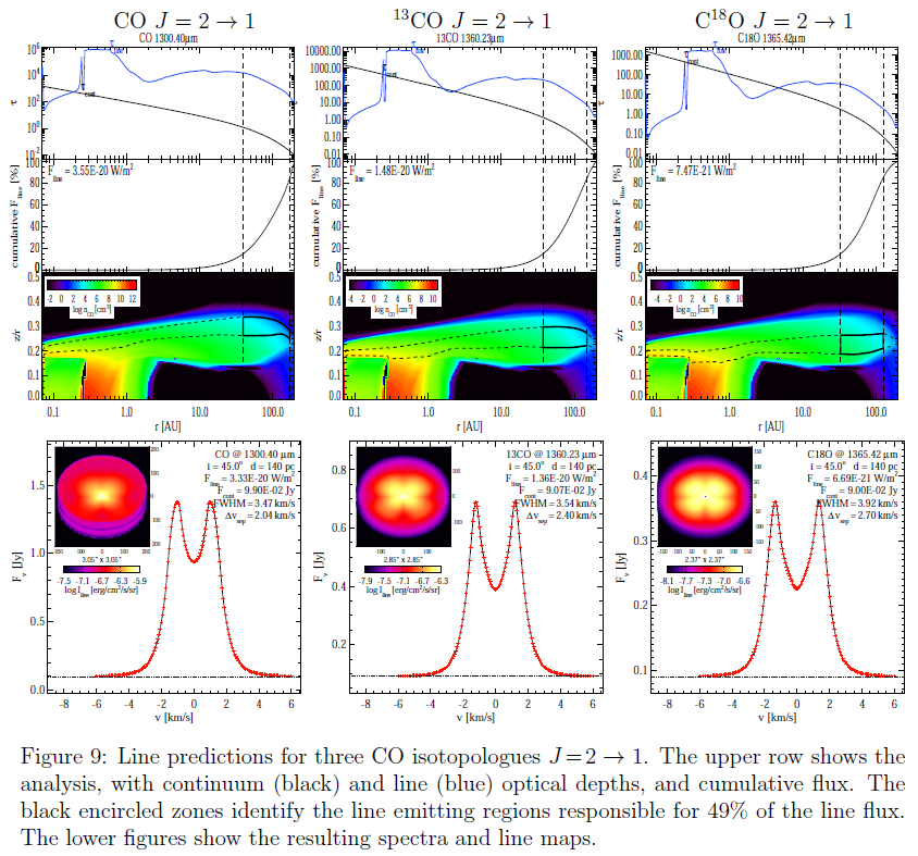
In Fig. 9 we see the results for the J = 2 → 1 lines of the three isotopologues CO, 13CO, C18O. Since these molecules have different abundances (assumed to be 1.0, 0.014, and 0.0020 with respect to CO, respectively), the lines in the series become less optically thick, are formed deeper and closer in, their FWHM and peak separation increases. The less abundant isotopologues form their lines in deeper layers, which makes the line ratio dependent on the vertical temperature gradients. These gradients, in return, depend on the assumption about the dust settling …
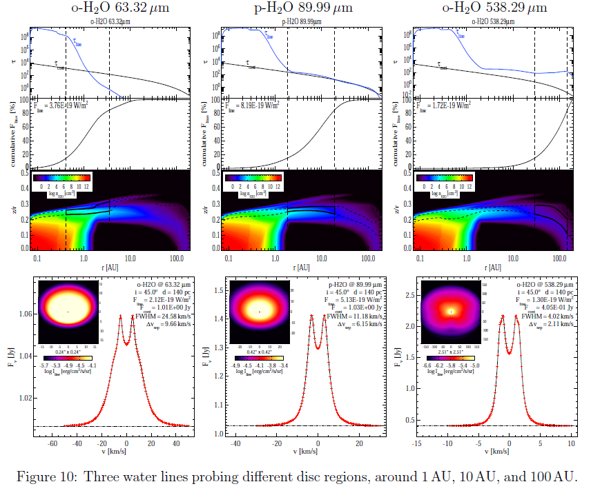
Figure 10 shows similar results for three selected water lines, which according to the model are emitted by completely different spatial regions of the disc. Trying a nebular analysis on these fluxes (e.g. deriving “the” rotational excitation temperature by a rotational diagram, assuming that all lines are emitted by the same gas with the same temperature) would obviously be quite misleading.
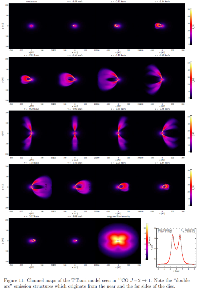
Figure 11 shows calculated channel maps for 13CO J = 2 → 1. One can see the much larger apparent size of the CO-disc (∼ 180 AU) as compared to the continuum (∼ 50 AU, upper left), although the local (column-integrated) gas/dust ratio is constant and equal to 100 by assumption in this model. The simple truth is that the CO molecular lines are still optically thick, even 13CO at 180 AU, where the continuum is already optically thin and vanishes in the background.
Return to:
1. Spectral Energy Distribution
2. Disc Shape and Dust Settling
3. Gas and Dust Temperatures
4. Chemical Structure
5. Predicted Continuum Observations